The Julia programming language provides some very powerful tools for modelling in systems biology. Not only is the language itself superb for scientific programming and heavy computations in general, its package ecosystem really makes systems biology easier to work with. Here, I will show the basic tools that I use when I model and simulate chemical reaction networks.

The most important package that I use is DifferentialEquations.jl. I would highly recommend anyone who computes differential equations in any form to read through this documentation thoroughly.

Model specification and simulation

Here, I will demonstrate a few ways of defining chemical reaction models, how to simulate them, and how to interact with final product. In all cases, we will use DifferentialEquations.jl to do most of the heavy lifting and if this tutorial piques you interest I would recommend that reading it’s documentation thoroughly.

Modelling using DiffEqBiological

DiffEqBiological.jl provides a domain-specific language (DSL) for chemical reaction modelling. In it’s main form, it supplies a macro that allow us to specify chemical reaction networks using a chemical arrow notation. Let’s have a look at a simple example:

using DiffEqBiological
model = @reaction_network begin
  r_f, a + b --> c
end r_f

Here, we are creating a model wherein the molecules $a$ and $b$ binds together (according to the law of mass action) with a forward binding rate $r_f$ to form the complex $c$. model is now a model instance which contains the mathematics needed to actually simulate the model. We can inspect the equations generated by this macro using the Latexify.jl package which will latexify the equations and try to render them for you:

using Latexify
latexify(model)

\begin{align} \frac{da(t)}{dt} =& - r_{f} \cdot a \cdot b \newline \frac{db(t)}{dt} =& - r_{f} \cdot a \cdot b \newline \frac{dc(t)}{dt} =& r_{f} \cdot a \cdot b \end{align}

We can also see that the model object holds a lot of pre-calculated information that can be used to speed up simulations. Here, for example, is the Jacobian:

latexify(jacobianexprs(model))

\begin{equation} \left[ \begin{array}{ccc}

r_{f} \cdot b & - r_{f} \cdot a & 0 \newline
r_{f} \cdot b & - r_{f} \cdot a & 0 \newline r_{f} \cdot b & r_{f} \cdot a & 0 \newline \end{array} \right] \end{equation}

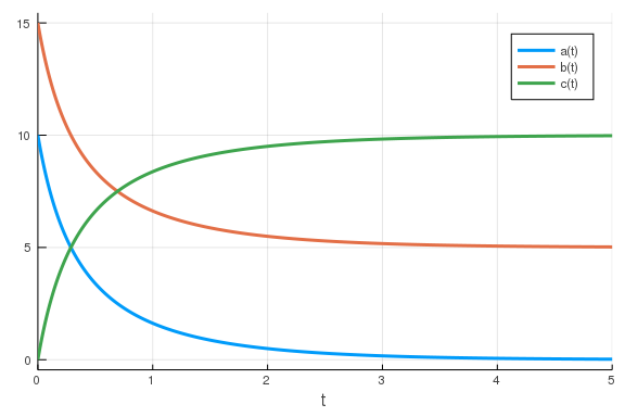
From here, it’s pretty simple to simulate our model. All we need to do is to define the parameter values, an initial condition and a timespan for the simulation before we call the relevant functions.

using DifferentialEquations

p = [0.2] # Vector of parameter values
u0 = [10., 15., 0.] # vector of initial concentrations
tspan = (0., 5.)

prob = ODEProblem(model, u0, tspan, p)
sol = solve(prob)

We have now simulated our model - yay! There are plenty of ways in which we could interact with the sol object (more info on that) but one of the most useful is plotting. This is really simple.

using Plots
plot(sol)

This is an example of how to perform a very simple simulation of a very simple chemical reaction model. We are, however, not restricted to such simple cases. We could define more complicated models which relies on more than just the law of mass action; we could solve these using stochastic differential equations (SDEs) or Gillespie simulations and we could add callbacks which triggers at certain events in the simulation and can alter its state, just to name a few. This quickly turns into a combinatorial problem where I don’t feel particularly inclined to demonstrate every possible combination. Instead, let’s just consider another case which utilises some of these tools.

Let’s study a positive feedback loop wherein two genes are mutually repressing the transcription of each other.

feedback = @reaction_network ModelPositiveFeedback η  begin
    hillR(y, v_x, k_x, n_x), 0 --> x
    hillR(x, v_y, k_y, n_y), 0 --> y
    (d_x, d_y), (x, y) --> 0
end v_x k_x n_x d_x v_y k_y n_y d_y

Here, we are seeing some additional functionality of the @reaction_netork macro. First of, this macro actually generates a new type. It did so in the previous example too, but here, we are specifying the name of that type to be ModelPositiveFeedback. Second, we are supplying a special noise-scaling parameter η. Third, we are using repressive Hill functions to regulate the production of x and y. Here, I should also mention that you can define arbitrary mathematical functions yourself which can be used in this framework, see here for details. Fourth, we are using a syntax wherein we specify the degradation of both x and y on the same line, each with its respective degradation rate. And, finally, we are specifying all the parameter names in the end. The order of these parameters is important to note since they determine which element of the parameter vector corresponds to which parameter.

Just like before, we can inspect the equations which are generated:

latexify(feedback)

\begin{align} \frac{dx(t)}{dt} =& \frac{v_{x} \cdot k_{x}^{n_{x}}}{k_{x}^{n_{x}} + y^{n_{x}}} - d_{x} \cdot x \newline \frac{dy(t)}{dt} =& \frac{v_{y} \cdot k_{y}^{n_{y}}}{k_{y}^{n_{y}} + x^{n_{y}}} - d_{y} \cdot y \end{align}

And, since we will be doing some stochastic simulations, we could also take the time to inspect the stochastic differential equations that are generated:

latexify(feedback; noise=true)

\begin{align} \mathrm{dx}\left( t \right) =& \left( \frac{v_{x} \cdot k_{x}^{n_{x}}}{k_{x}^{n_{x}} + y^{n_{x}}} - d_{x} \cdot x \right) \cdot dt + \eta \cdot \sqrt{\left|\frac{v_{x} \cdot k_{x}^{n_{x}}}{k_{x}^{n_{x}} + y^{n_{x}}}\right|} \cdot dW_{1(t)} -1 \cdot \eta \cdot \sqrt{\left|d_{x} \cdot x\right|} \cdot dW_{3(t)} \newline \mathrm{dy}\left( t \right) =& \left( \frac{v_{y} \cdot k_{y}^{n_{y}}}{k_{y}^{n_{y}} + x^{n_{y}}} - d_{y} \cdot y \right) \cdot dt + \eta \cdot \sqrt{\left|\frac{v_{y} \cdot k_{y}^{n_{y}}}{k_{y}^{n_{y}} + x^{n_{y}}}\right|} \cdot dW_{2(t)} -1 \cdot \eta \cdot \sqrt{\left|d_{y} \cdot y\right|} \cdot dW_{4(t)} \end{align}

Here, we se that we are using the chemical Langevin equations and that each reaction has an independent noise term.

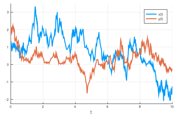
So, lets simulate this using SDEs.

u0 = [1., 2.]

## parameter order: v_x k_x n_x d_x v_y k_y n_y d_y η
p = [1, 0.5, 2, 1, 1, 0.5, 2, 1, 1]
tspan = (0., 10.)
sde_prob = SDEProblem(feedback, u0, tspan, p)
sol = solve(sde_prob)

plot(sol)

So, we have already performed a stochastic simulation, cool! We do, however, have a bit of a problem: the concentrations are sometimes negative. This does not make sense from a chemical/biological point of view. It is a consequence of us using a noise approximation which is inaccurate for low copy-numbers of the molecules. What low copy-numbers in this case means is a little bit unclear since have chosen to interpret the variables x and y as concentrations. A better way of thinking about it is that we run in to problems whenever concentrations are low relative to the noise. In some cases, the issue could be remedied either by rescaling the concentrations to have higher values or by rescaling the noise to have a lower amplitude. In order to get a “true” ratio between these, we would have to specify the model more strictly and define what volume our simulated molecular concentrations are in. Often, the true values of this (and a lot of other model parameters) are inaccessible to us. A way to circumvent this could be to consider the noise scaling parameter, $\eta$, to be a free parameter which is fitted to data. 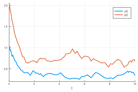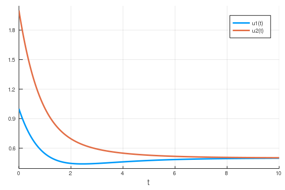Since we are currently only looking at what tools Julia can provide us with, I will simply drop this reasoning here, content that I have warned you, and just show what happens when you reduce the noise parameter.

p[end] = 0.1
sde_prob = SDEProblem(feedback, u0, tspan, p)
sol = solve(sde_prob)

plot(sol)

That did make a difference!

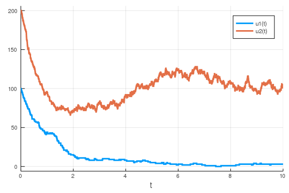
The chemical Langevin equations holds well as long as copy-numbers are large enough but sometimes the model says that they should tend to zero. In this case the SDE apporach is doomed to have some inaccuracies. A more correct, but potentially much slower, way of simulating this would be to use a Gillespie simulation. In such case, our variables x and y will not be representing concentrations but rather the number of the respective molecules. We therefore have to rescale the initial conditions and parameter values a bit before we can run a simulation that makes any sense.

u0 = [100, 200] # Now, we are using the number of molecules instead of concentration.

p = [50., 30, 2, 1, 100., 30., 2, 1, 1]

prob = DiscreteProblem(u0, tspan, p)
jump_prob = JumpProblem(prob, Direct(), feedback)
sol = solve(jump_prob)

plot(sol)

I did call this slow but I think that I have to qualify what that means. We can examine how long it actually took to simulate the models:

using BenchmarkTools
@btime solve(sde_prob);

71.375 μs (1044 allocations: 49.64 KiB)

@btime solve(jump_prob);

519.710 μs (3448 allocations: 522.22 KiB)

Here, we do see a factor five performance difference, but really, they are both blazingly fast. If you can even notice any lag when executing the code it is due to the plotting, not the solving. However, the two approaches scale differently with the complexity and the separation of time-scales within the simulations. There are cases where the performance difference becomes significant. Still, this is normally not prohibitive for simulating a model, the real issue starts when you want to repeat the simulations tens of thousands of times during parameter optimisation (we’ll get to that later).

A another feature that I would like to showcase is the use of callbacks. With callbacks, you can specify some criterion at which the simulation should pause and where you can alter the state of the simulation before you let it continue. A simple example of this would be to stop at a given time and change a parameter or variable value. I often do this to represent some event which occurred in an experiment who’s results I’m trying to capture with the model.

u0 = [1., 2.]

## parameter order: v_x k_x n_x d_x v_y k_y n_y d_y η
p = [1, 0.5, 2, 1, 1, 0.5, 2, 1, 1]
tspan = (0., 10.)

affect!(integrator) = (integrator.p[1] *= 5)
tstop = 5
callback = PresetTimeCallback(tstop, affect!)

sde_prob = ODEProblem(feedback, u0, tspan, p)
sol = solve(sde_prob; callback=callback)

plot(sol)

This is a simple example but the world is your oyster. Callbacks can be used for any type of simulation and you could use it do something crazy - like tripling the concentration of anything that decreases below a given value:

u0 = [1., 2.]

p = [1, 0.5, 2, 1, 1, 0.5, 2, 1, 1]
tspan = (0., 10.)


function condition(out, u, t, integrator)
	out .= u .- 0.5
end

function affect!(integrator, event_index)
    integrator.u[event_index] *= 3
end
tstop = 5
callback = VectorContinuousCallback(condition, affect!, length(u0))

sde_prob = ODEProblem(feedback, u0, tspan, p)
sol = solve(sde_prob; callback=callback)

plot(sol; ylims=(0., Inf))

Sometimes the use of the @reaction_network macro can be limiting since it is rather static. If you, for example, would like to programmatically build your model using loops and such, there is another way to go about it. To spare myself some typing I’ll simply refer you to this nice tutorial if you’re interested in this.

So, we have now seen how to use DiffEqBiological.jl to specify models and how to simulate these in different ways. This is a very convenient way of introducing the subject since it allows me to demonstrate a lot of features even though the code is still small and easy to understand. However, I still find that there are cases where DiffEqBiological.jl is not the best available option for modelling and I will, therefore, describe some others as well.

Alternative methods of modelling chemical reaction networks

There are other ways of generating a mathematical model of reaction networks than to use DiffEqBiological.jl. Here, I will mention three alternatives, two of which relies on some domain-specific language (DSL) to do much of the work for you and the other one is to simply define all the necessary functions yourself. Of the three, I would say that the do-it-yourself method is the most important one to know so I’ll only briefly introduce the other two.

Specifying models using ParameterizedFunctions.jl

ParameterizedFunctions.jl supplies a macro, @ode_def, which allows you to input a set of ordinary differential equations in a manner which looks very much like it would if you jotted it down on paper.

using ParameterizedFunctions

ode_model = @ode_def MyModel begin
    dx = v_x * k_x / (k_x + y) - d_x * x
    dy = v_y * k_y / (k_y + x) - d_y * y
end v_x k_x d_x v_y k_y d_y

latexify(ode_model)

\begin{align} \frac{dx}{dt} =& \frac{v_{x} \cdot k_{x}}{k_{x} + y} - d_{x} \cdot x \newline \frac{dy}{dt} =& \frac{v_{y} \cdot k_{y}}{k_{y} + x} - d_{y} \cdot y \end{align}

This model can be simulated in almost exactly the same way as a model from DiffEqBiological.jl. The only difference is that this macro does not define the equations necessary for stochastic simulations.

Specifying models using ModelingToolkit.jl

I won’t actually go into any details at all here, I just want to mention that this exists. While it sort-of works at the time that I’m writing this, I still find it very immature and a bit buggy. At some point, I think that this package will become highly important but I would not recommend it to a beginner today. However, you might not be reading this post ‘today’ (2019-11-01) so it might be worth having a look here.

Specifying models from scratch

You can simulate an ODE straight from a function that specifies the model’s derivatives. The function must take either three (u, p, t) or four arguments (du, u, p, t), in that order. In the first case, the function must return a vector of the derivatives and in the second case, the function must mutate the derivative vector, du (this is usually faster).

function model_derivs(du, u, p, t)
    du[1] = p[1] * p[2] / (p[2] + u[2]) - p[3] * u[1]
    du[2] = p[4] * p[5] / (p[5] + u[1]) - p[6] * u[2]
end

u0 = [1., 2.]
p = [1, 0.5, 1, 1, 0.5, 1]
tspan = (0., 10.)
prob = ODEProblem(model_derivs, u0, tspan, p)
sol = solve(prob)
plot(sol)

This puts all of the power, and all of the responsibility, in your hands. No extras are computed, such as the Jacobian or the noise equations. All of this (and more) can be created manually, but its all up to you to do so. An advantage of this is that it may be easier to utilise loops and such. This is particularly advantageous if the number of variables in your model depends on the input (u or p) as it could do for spatial simulations for example. Again, showcasing all of this would simply take too long and since the documentation is excellent, I’ll just refer you there.

Parameter fitting

I use BlackBoxOptim.jl for parameter fitting. It’s an optimisation package that supplies global optimisation algorithms that does not require you to specify the gradients of your problems.

In order to do parameter fitting (or parameter optimisation as it is also called) you need to have a function which computes how well the model met its target with a given parameter set.

To showcase this, let’s generate some synthetic data from a model and then see if we can optimise a new model to fit that data.

datamodel = @reaction_network begin
    r_1, x_1 --> x_2
    r_2, x_2 --> x_3
    r_3, x_3 --> 0
end r_1 r_2 r_3

u0 = [100., 0., 0.]
p = [1., 2., 3.]
tspan = (0., 10.)

prob = ODEProblem(datamodel, u0, tspan, p)
sol = solve(prob)

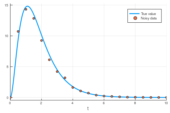
sample_times = 0.:0.5:10
data = sol.(sample_times; idxs=3)

## Add some noise to the data
data .*= 1 .+ 0.3 .* (rand(length(data)) .- 0.5)

## Plot the true solution and the noisy data.
plot(sol; vars=3, label="True value")
scatter!(sample_times, data; label="Noisy data")

Now we have some data but we need to specify some cost function which measures how good a model + parameter set is at reproducing the data. Let’s say that we have the slightly incorrect hypothesis that the data was generated by a system which looks like:

model = @reaction_network begin
    r_1, x_1 --> x_2
    r_2, x_2 --> x_3
    r_3, x_3 --> x_4
    r_4, x_4 --> 0
end r_1 r_2 r_3 r_4

Let’s also say that we know that the initial concentration of $x_1$ should be $100$ and that the rest should be zero. We’ll take the models last variable to be the one which should match the data and we write the following functions:

function cost(parameters)
    ## First we need to simulate the model with the parameters
    u0 = [100., 0., 0., 0.]
    tspan = (0., 10.)

    prob = ODEProblem(model, u0, tspan, parameters)
    sol = solve(prob)

    ## Extract the values that we wish to compare to the target
    result = sol.(sample_times; idxs=4)

    ## Calculate the square distance to the data
    cost = sum((result .- data) .^ 2)

    return cost
end

cost (generic function with 1 method)

This function reduces a parameter set to a single cost value which the optimiser will try to minimise. The function will work and is a good first demonstration, but I should warn you that it is very poorly written (we’ll return to that in a different post).

We can now perform our parameter fitting:

using BlackBoxOptim
result = bboptimize(
    cost; 
    SearchRange=(0., 100.), 
    NumDimensions=numparams(model)
    );

Starting optimization with optimizer BlackBoxOptim.DiffEvoOpt{BlackBoxOptim
.FitPopulation{Float64},BlackBoxOptim.RadiusLimitedSelector,BlackBoxOptim.A
daptiveDiffEvoRandBin{3},BlackBoxOptim.RandomBound{BlackBoxOptim.Continuous
RectSearchSpace}}
0.00 secs, 0 evals, 0 steps
0.50 secs, 2141 evals, 2038 steps, improv/step: 0.265 (last = 0.2650), fitn
ess=2.371503648
1.00 secs, 4233 evals, 4130 steps, improv/step: 0.212 (last = 0.1611), fitn
ess=0.729849718
1.50 secs, 5911 evals, 5808 steps, improv/step: 0.213 (last = 0.2139), fitn
ess=0.664729539
2.00 secs, 7276 evals, 7173 steps, improv/step: 0.216 (last = 0.2300), fitn
ess=0.662892317
2.50 secs, 8613 evals, 8510 steps, improv/step: 0.218 (last = 0.2259), fitn
ess=0.661408397

Optimization stopped after 10001 steps and 2.97 seconds
Termination reason: Max number of steps (10000) reached
Steps per second = 3363.75
Function evals per second = 3398.39
Improvements/step = 0.21570
Total function evaluations = 10104


Best candidate found: [0.82783, 3.23866, 99.9967, 3.03868]

Fitness: 0.661288464


opt_params = best_candidate(result)

4-element Array{Float64,1}:
  0.8278295081233895
  3.2386645577478785
 99.996660391062    
  3.0386759698782453

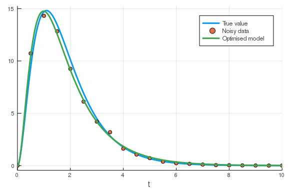
u0 = [100., 0., 0., 0.] 
tspan = (0., 10.)

prob = ODEProblem(model, u0, tspan, opt_params)
sol = solve(prob)

## plot the solution on top of the data-plot
plot!(sol; vars=4, label="Optimised model")

Conclusion

Here, we have the fundamental tools that I use for modelling in systems biology. I’m hoping that this is sufficient to get people not only started but also enthusiastic about starting.

In a future post, I will dig a lot deeper into how I would organise code and data for a large-ish research project such that everything becomes modular and easy to use and extend. There, we will see the power of using specialised types, multiple dispatch and plot recipes.

Modelling systems biology using Julia - the basics

Powerful modelling in a terse and intuitive language