Here, I will discuss the mapping between the parameters of simplified linear pathway models and the fully enumerated system and the data produced thereof. I will show how the parameters can be estimated analytically through measurements (or prior knowledge) of the mean and the variance of the time at which an output signal is observed. This is then compared to the slower, but more resilient, method of using numerical optimisation. Along the way, we will also gain insight into the reverse problem; given a model with fitted parameters, what can we say about the biological pathway that the model is representing?
In our recent paper preprint we (me and my PhD supervisor) explore how to represent the action of linear biochemical pathways with simple models. We show that such pathways lead to dynamics that can accurately and succinctly be recaptured by simplified models wherein one has assumed that the rate of information transfer along the pathway is fixed and homogeneous. Such an assumption, even if false, reduces the representation of arbitrary linear pathways to a small model with only three free parameters. The accuracy of such models far surpasses models utilising the more common simplification technique of effectively shortening the pathway length in the model as compared to reality.
Before continuing, I should quickly clarify what I mean by a linear pathway. What I mean is a pathway that is both topologically linear - a straight line of successive reactions - and linear in how the previous pathway step activates the next (first order kinetics).
The first step in the pathway receives some input, I(t), and the $n$-th pathway step is considered to be the output of the pathway.
Assuming that their dynamics can be represented with deterministic and continuous equations we can write
\begin{align}
X_1 =& p_1 \cdot I(t) - d_1 \cdot X_1 \\
X_i =& p_i \cdot X_{i-1} - d_i \cdot X_i \quad \forall i \in {2, 3, …, n}\\
\end{align}
where $p$ and $d$ are production/activation and degradation/dilution/inactivation rates, respectively.
In the paper, this fixed-rate assumptions leads us to an analytical model that accurately represents the dynamics of arbitrary linear pathways after a unit impulse input, \begin{equation} X_n^{real}(t) \approx g(t) = \gamma \cdot \underbrace{\frac{ \beta^{\alpha} \cdot t^{\beta - 1} \cdot e^{ - \beta \cdot t}}{\Gamma\left( \alpha \right)}}_{\textrm{Gamma distribution PDF}}. \end{equation} Here, we approximate the dynamics of $X_n^{real}(t)$ which is the output the “real” linear pathway, with $n$ reaction steps that all occur at arbitrary and independent rates, $r_i$. $\alpha$ is the “shape parameter” and $\beta$ the “rate parameter” of the gamma distribution, which here are related to the pathway length and the reaction rates of the pathway, respectively (in the paper these parameters are denoted $n$ and $r$). $\gamma$ is a parameter that governs how the input signal is scaled (amplified or dampened) before it generates an output.
The scope of this precise model is limited to representing pathways which starts out fully inactive but which receives a unit impulse, $\delta(t)$, at $t=0$. This may seem like an unreasonable constraint that renders it practically useless but that is not the case, for two reasons. First, these conditions can represent dormant signalling pathways with a non-zero concentration of the first pathway step that is suddenly released upon some external cue. This could for example represent signal pathways within the immune system, as we shall soon see. Second, by using these conditions we have ensured that the above equation represents the transfer function (see wikipedia or Ogata’s freely available book on control theory). If we know the transfer function, $g(t)$, we can get the dynamics for arbitrary inputs from the convolution of it and the input, $I(t)$, \begin{equation} X_n^{real}(t) \approx g(t) * I(t) = \int_0^\infty g(t - \tau) \cdot I(\tau) d\tau. \end{equation}
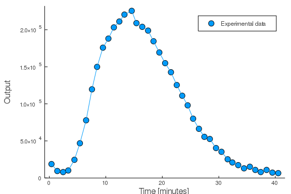
The paper argues for the validity of such a modelling approach but here we will turn our focus to some more practical matters of usage and, particularly, parameter fitting. For this, we’ll use a real example from the immune response of Arabidopsis Thaliana. Receptors on the surface of the plant leaves detects incoming pathogens or other signals of danger and triggers a pathway which results in the release of reactive oxygen species. Upon a sudden but persistent experimental application of the input, the time-course of the output was measured (Monaghan et al. 2014, Col-0 of figure 3a):
 \
\
So, how do we go about fitting the model to this data? First, we postulate that the presence of the input “releases” some initial reservoir of immune responders into a previously dormant pathway, allowing us to represent the dynamics directly using $g(t)$. Then, when we now have decided which model to use, we need to find the appropriate parameters of that model. We will do this in two different ways, one relying on a statistics-based argument and one relying on numerical optimisation.
Parameters estimation from means and the variances
The statistics-based argument arises from the fact that the model, $g(t)$, closely follows the probability density function of the gamma distribution. The random variable in this distribution is time - the time it takes for a single input particle to result in a single output particle. For the gamma distribution, the mean of this time is given by [ \langle t_{g} \rangle = \frac{\alpha}{\beta} ] and the variance is given by
[
\sigma^2_{t_g} = \frac{\alpha}{\beta^2}.
]
While it is not reasonable to expect the model to fit the data perfectly in all respects, it could be reasonable to demand that the mean and the variance of the time it takes for the input to generate an output should be the same for the model and the data. This demand can be stated as
\begin{align}
\langle t_{data} \rangle =& \langle t_{g} \rangle = \frac{\alpha}{\beta} \\
\sigma^2_{t_{data}} =& \sigma^2_{t_g} = \frac{\alpha}{\beta^2}.
\end{align}
With some rearranging, these two equations gives us expressions for the parameters $\alpha$ and $\beta$ in terms of the mean and the variance of the data:
\begin{align}
\alpha =& \frac{\langle t_{data} \rangle^2}{\sigma^2_{data}}\\
\beta =& \frac{\langle t_{data} \rangle}{\sigma^2_{data}}\\
\end{align}
Here, we have an analytical estimation of the “optimal” model parameters, based on the assumption that the fit is optimal if the mean and the variance of the model matches that of the data.
So, how and when do we use this? Essentially, the crude answer is that we can use this approach when it is available and when seems to work well for us. The method is only available if we can estimate/calculate the required statistics from data/the data-generating model. And ‘it working well’ is contingent both on how this definition of optimality aligns with our goals and on how well we can estimate the required statistics from data.
Estimating parameters for PDF-like data.
The case where this parameter estimation method can most easily be applied is when the data is expected to trace the outline of a probability density function (PDF).
This is expected for time-courses which tracks the output of a linear pathway after the application of certain kinds of input.
One such input is the impulse input wherein the input only exists for a negligible amount of time but still manages to trigger a significant response.
 \
\
I struggle to come up with known cases where this would apply but one could imagine it being some mechanical blow, for example.
A more realistic input is the exponentially decaying one.
 \
\
Here, one could imagine the input being some added concentration of molecules which decays or is diluted with some fixed half-life (not at all uncommon).
One would then have to consider the input to actually be the first step in the pathway when one considers the length, $n$, of the pathway.
A third scenario where the data is expected to trace a PDF is when a step-input (which changes from 0 to a constant value and stays at that value) triggers the conversion and depletion of an initial molecule which is not quickly replenished.
 \
\
This last scenario is indeed what we think is happening for the experimental data in our example. A constant amount of input is applied, the first step of the pathway is being used up and it is only replenished on a timescale of a full day while the observed dynamics occurs during less than an hour.
The mean and variance of a distribution with a PDF $f(t)$ ($f(t)=0 ; \forall t < 0$) can, respectively, be calculated with
\begin{align}
\langle t \rangle =& \int_0^\infty t \cdot f(t) dt \\
\sigma^2_{t} =& \int_0^\infty (t - \langle t \rangle)^2 \cdot f(t) dt.
\end{align}
The data that we are using will, typically, not follow the PDF but rather a scaled version of the PDF which we can call $y(t)$. To get the PDF from this scaled function we would have to normalise it:
\begin{align}
f(t) = \frac{y(t)}{\int_0^\infty y(t) dt}.
\end{align}
Incidentally, this normalisation faction directly gives us the $\gamma$ parameter for the gamma model.
In the simple case of our samples being take at a fixed time interval, $\Delta t$, we can approximate the values of these statistics with
\begin{align}
\langle t_{data} \rangle \approx& \frac{\sum_{i=1}^{N} \left( y_i \cdot t_i \right)}{\sum_{j=1}^{N} y_j}\\
\sigma^2_{t_{data}} \approx& \frac{\sum_{i=1}^{N} \left( y_i \cdot (t_i - \langle t_{data} \rangle)^2 \right)}{\sum_{j=1}^{N} y_j}\\
\end{align}
Here, $y_i$ and $t_i$ are the values and time-points for each data point in time trajectory data of interest.
If one needs a better approximation than this, or if one has data which is not sampled regularly, one can instead interpolate the data to approximate $y(t)$ and use this to actually solve the integrals above.
By estimating of the mean and the variance of the data and plugging it in to the equations for $\alpha$ and $\beta$, we can easily calculate their “optimal” values. Here, this results in a pretty convincing model/data fit.
 \
\
So, this parameter estimation technique sometimes works very well and a computer can do it just about instantaneously, but there are cases when it does not work as well. Another time-course from the same paper seems less amenable to this method of parameter estimation.
 \
\
Here, the data seems rather more noisy and I suspect that the noisy tails of the outlined PDF impacts the fit. We should point out that he presumed noise is bad enough for us to think that no solution would ever have a strikingly good fit. However, this particular fit is even so a bit lacking.
Estimating parameters for CDF-like data.
Another kind of data which can be estimated using this statistics-based approach is those that are outlining a cumulative density function.
This is something that we would expect from a time-course wherein for example a step input provides a constant source of signalling to a pathway with steps that are not depleted by the process.
 \
\
It could also be that the step input releases the flow of signalling from the first step of the pathway to the rest. Unlike for the PDF case, however, the first step would here have to be either rapidly replenished or not used up in the activation of the next step.
 \
\
The time-course of such a system is distinguishable from those that follow a PDF in that they reach a maximal level of signalling and stays there.
Given a CDF, $F(t)$, the mean can be calculated by
\begin{equation}
\langle t \rangle = \int_0^\infty 1 - F(t) dt = \int_0^\infty t \cdot \frac{F(t)}{dt} dt \\
\end{equation}
Again, data is not likely to track the CDF directly, but rather a scaled version of it $Y(t)$ which relates to the CDF by
\begin{equation}
F(t) = \frac{Y(t)}{Y(\infty)}
\end{equation}
To get the variance, we can use that \begin{equation} \sigma^2 = \langle t^2 \rangle - \langle t \rangle^2 \end{equation} where we can get $\langle t^2 \rangle$ from
\begin{equation} \langle t^2 \rangle = \int_0^\infty 2 t \cdot \left(1 - \frac{Y(t)}{Y(\infty)} \right) dt. \end{equation}
Here, we’d need to approximate $Y(\infty)$ from the data. This may or may not be trick. This value is simply the concentration that the output is asymptotically approaching. In noise free data, one could simply use the last value of the time-series, given that the series went on long enough for the output to plateau. With noisy data, one could try to use the mean of all the data points acquired late enough that they appear to have reached this asymptote. Regardless of how you estimated it, let’s call it $y_{\infty}$.
Again, for the simple case of the time course being sampled at equal intervals, $\Delta t$, we can approximate the mean and the mean of the squares by
\begin{align}
\langle t_{data} \rangle \approx& \Delta t \cdot \sum_{i=1}^{N} \left(1 - \frac{y_i}{y(\infty)} \right) dt \\
\langle t_{data}^2 \rangle \approx& \Delta t \cdot \sum_{i=1}^{N} 2 \cdot t_i \cdot \left(1 - \frac{y_i}{y(\infty)} \right) dt.
\end{align}
The variance can be estimated by $\sigma^2 = \langle t_{data}^2 \rangle - \langle t_{data} \rangle^2$ but here we see a potential problem. The error in our estimates of the mean and of $y_\infty$ are squared. This means that if our estimates are a bit off, the final result can end up being fairly bad.
Anyway, we generated a bit of synthetic data from a step input, added some noise to the output, and tried to use our method to fit the gamma model.
To make things harder, we did not “sample” the “data” homogeneously so we had to resort to using integrating interpolated data.
 \
\
Not bad. We have, however, cherry-picked a little bit.
Parameter estimation using numerical optimisers
An alternative technique for parameter estimation is to simply use a numerical optimiser. This involves defining a cost function which compares the model to the data and returns a single value that decreases as the model/data fits increases. There is many ways of defining a cost function and the definition matters since it is essentially defining what optimality is. A common cost function is the sum of squares, but we have opted to instead minimise the area mismatch between the model and the data output curve (this is defined in the paper). Then we need to find an optimisation algorithm to minimise that cost function. Numerical optimisation is an entire research field in itself but there are generally some good libraries available in the programming language of your choise. We used a differential evolution scheme implemented in BlackBoxOptim.jl for the Julia programming language. For these very simple examples, the numerical optimisation only took a few seconds and the resulting fits are shown:
 \
\
Here, I would say that the numerical optimisation provides a better model/data fit. It is a bit hard to argue this point since both of the fits are (near) optimal but with different definitions of what optimality means. It comes down to what parts of the dynamics one wish the model to preserve and what parts of the data one trusts to be accurate. For the right figure, where the two methods differ in results, I would prefer how the numerical fit preserves more of the shape of the output curve. I would also trust the low valued data points less than the others due to their noise sensitivity. Picking between two definitions of optimality is however a bit arbitrary.
Arbitrary choices aside, the model still fits the data very well. The model greatly simplifies reality and allows a three-parameter representation of the biological pathway underlying the data. Its parameters can easily be estimated numerically or using simple statistics of the data. As we show in the paper, these optimal parameter values are also revealing about the properties and the structure of the pathway that generated the data. The model is accurate and easy to use, either in the form presented here or in its pure differential equation from. For more information read the paper.